Step-by-step guide#
This guide shows step by step how a compartmental model is built and how its parameter can by inferred.
First some imports
[1]:
import time

import arviz as az
import jax
import jax.numpy as jnp
import jaxopt
import matplotlib.pyplot as plt
import numpy as np
import optax
import pymc as pm
import pytensor.tensor as pt
from tqdm.auto import tqdm

import icomo
Let us first define a system of ordinary differential equations (ODEs). As an example, we will make an SEIR model with an Erlang distributed latent period.
[3]:
# ODEs should always be defined with t, y and args, t is the time variable, y the
# variables proper and args the other arguments
def Erlang_SEIR(t, y, args):
    # args can be time dependent or not, if there are time-dependent variable, args
    # is passed as a tuple, where the first entry beta_t is a function that can be
    # evaluated at t
    beta_t, const_arg = args

    # y and the other constant args are passed as dictionary in this example to facilite
    # keeping track of the meaning of the variables
    N = const_arg["N"]
    dy = {}  # Create the return dictionary of the derivatives, it will have the same
    # structure as y

    # The derivative of the S compartment is -beta(t) * I * S / N
    dy["S"] = -beta_t(t) * y["I"] * y["S"] / N

    # Latent period, use an helper function
    dEs, outflow = icomo.erlang_kernel(
        inflow=beta_t(t) * y["I"] * y["S"] / N,
        Vars=y["Es"],  # y["Es"] is assumed to be a list of compartments/variables to be
        # able to model the kernel
        rate=const_arg["rate_latent"],
    )
    dy["Es"] = dEs

    dy["I"] = outflow - const_arg["rate_infectious"] * y["I"]

    dy["R"] = const_arg["rate_infectious"] * y["I"]

    return dy  # return the derivatives
The above function defined the following set of equations:
Here \(n = 3\) is the number of exposed compartments \(E\). In the function above the exposed compartments are saved as list in y["Es"]. The three equations \(\frac{\mathrm dE^{(1 \dots 3)}(t)}{\mathrm dt}\) are defined in the icomo.erlang_kernel function for convenience. This function also sets dynamically \(n\) to the length of the list y["Es"]. Take care to only use jax operations inside the differential equation, for
instance jnp.cos instead of np.cos. It will be compiled with jax later and would otherwise lead to an error.
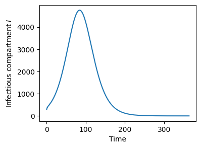
Integrating ODEs#
Given some starting conditions and parameters we can integrate our system of ODEs:
[4]:
len_sim = 365  # days
num_points = len_sim

### First set the time variables
t_out = np.linspace(0, len_sim, num_points)  # timepoints of the output
t_solve_ODE = np.linspace(0, len_sim, num_points // 2)  # timepoints at which the ODE
# is solved
t_beta = np.linspace(
    0, len_sim, num_points // 14
)  # timepoints at which the time-dependent
# variable is defined (every 2 weeks)

### Define parameters
N = 1e5  # population
R0 = 1.5
duration_latent = 3  # the average in days
duration_infectious = 7  # the average in days
beta0 = R0 / duration_infectious  # infection rate


### Set parameters  for ODE
arg_t = beta0 * np.ones(len(t_beta))  # beta might be time-depedent, but assume
# constant beta for now
const_args = {
    "N": N,
    "rate_latent": 1 / duration_latent,
    "rate_infectious": 1 / duration_infectious,
}

### Define starting conditions
y0 = {
    "Es": [100, 100, 100],  # multiple compartmentes for Erlang kernel
    "I": 300,
    "R": 0,
}
# Susceptible compartment is N - other compartments
y0["S"] = N - jax.tree_util.tree_reduce(lambda x, y: x + y, y0)
# This is equivalent to writing
y0["S"] = N - y0["R"] - np.sum(y0["Es"])


# First parameters of the integrators have to be set
integrator_object = icomo.ODEIntegrator(
    ts_out=t_out,
    t_0=min(t_solve_ODE),
    ts_solver=t_solve_ODE,
    ts_arg=t_beta,
)

# Then we can obtain a function that solves our system of ODEs
SEIR_integrator = integrator_object.get_func(Erlang_SEIR)

# And solve the ODE for our starting conditions and parameters
output = SEIR_integrator(y0=y0, arg_t=arg_t, constant_args=const_args)

f = plt.figure(figsize=(4, 3))
plt.plot(output["I"])
plt.xlabel("Time")
plt.ylabel("Infectious compartment $I$");

We here use an ODE integrator built with the icomo.ODEIntegrator which wraps the ODE solver from Diffrax. In general, the constant_args and variables y0 passed to the integrator and subsequently to the ODE function can be a any nested list, tuple and/or dict, which is also called pytree. The output will have the same structure as y0 except that
its variables will received a prependet time dimension. arg_t has to be an ndimensional array, where the first dimension matches the length of ts_arg.
Simplify the construction of ODEs with icomo.CompModel#
The system of ODEs can by vastly simplified. Notice how the population subtracted from one compartment is always added exactly to another compartment. Furthermore, the substracted amount is always proportional to the population currently in the compartment. Making use of these two properties, one can specify such a system by a number of flows starting and ending in different compartments and parametrized by rates which are multiplied by the starting compartment. Such a spefication is possible with the class icomo.CompModel:
[5]:
def Erlang_SEIR_v2(t, y, args):
    beta_t, const_arg = args

    comp_model = icomo.CompModel(y)

    comp_model.flow(
        start_comp="S",
        end_comp="Es",
        rate=y["I"] / const_arg["N"] * beta_t(t),
        label="beta(t) * I/N",  # label of the graph edge
        end_comp_is_list=True,
    )  # One has to specify that "Es" refers to
    # a list of compartments
    comp_model.erlang_flow(
        "Es", "I", const_arg["rate_latent"], label="rate_latent (erlang)"
    )
    comp_model.flow("I", "R", const_arg["rate_infectious"], label="rate_infectious")
    comp_model.view_graph()
    return comp_model.dy


# Check whether the resulting dynamics are the same as the previous version
SEIR_integrator_v2 = integrator_object.get_func(Erlang_SEIR_v2)
output2 = SEIR_integrator_v2(y0=y0, arg_t=arg_t, constant_args=const_args)

f = plt.figure(figsize=(4, 3))
plt.plot(output2["I"])
plt.xlabel("Time")
plt.ylabel("Infectious compartment $I$");


Another advantage is the a CompModel object can display the graph with the view_graph() method, which helps the verify the parametrisation was correct. Specify in this case the label keyword when adding flows, these are displayed on the edges of the graph.
Take notice that CompModel assumes that the variables/compartments y are saved in a dictionary and that for flow that follow and Erlang kernels, the corresponding compartments are in a list saved under the key of `start_comp.
Fitting/optimizing the model using Data#
We might to optimize some parameters of the model. This is readily achieved as it can be easily differenciated using jax.grad.
Concretely, we will optimize the beta_t variable. We defined it every 14 days. The icomo.ODEIntegrator class uses a cubic interpolation to obtain a continuous approximation inbetween. For completeness, we will also need to optimize the initial number of infected I0.
[6]:
# Data are the number of COVID-19 cases in England during 2022
data = [236576, 188567, 118275, 181068, 229901, 275647, 222174, 172980, 120287, 93615, 95790, 132959, 115245, 103219, 96412, 86325, 77950, 98097, 131514, 118857, 111760, 100324, 91730, 81733, 102365, 127364, 113201, 108668, 96200, 84026, 73512, 87702, 105051, 93949, 88418, 76644, 63264, 52305, 60552, 76483, 69661, 64339, 52293, 44559, 37529, 41755, 54745, 52502, 51572, 44716, 33241, 34647, 37720, 45131, 39188, 36476, 30631, 27837, 25089, 31360, 44649, 44795, 46179, 43761, 41408, 38759, 49026, 68520, 70111, 73531, 70510, 67030, 62078, 75738, 99832, 93708, 91752, 82853, 75285, 67417, 81054, 109286, 99095, 94185, 82905, 72430, 61456, 68336, 92857, 80126, 73643, 54791, 47462, 37592, 42179, 53727, 49101, 44750, 38709, 32988, 27885, 30952, 37371, 33771, 31685, 26638, 21615, 19924, 20144, 25223, 25772, 21457, 18464, 15703, 13210, 14715, 17108, 14560, 13055, 11608, 10012, 8354, 9034, 11907, 13318, 11672, 10221, 8954, 7517, 9062, 10702, 9748, 8725, 7642, 6942, 6120, 7973, 9417, 8286, 7638, 6820, 5821, 5019, 5997, 7313, 6679, 6293, 5753, 5409, 4988, 5680, 7115, 7093, 7011, 6209, 6635, 7492, 9815, 11747, 11411, 11784, 11319, 10784, 10077, 12693, 15272, 15141, 14837, 14225, 13919, 13623, 16997, 19942, 20896, 20873, 19590, 18349, 16800, 20778, 25104, 25041, 24601, 24240, 23650, 21961, 27780, 33704, 31415, 29698, 26454, 24611, 21246, 25096, 29826, 26946, 23856, 21100, 18359, 15017, 17236, 18718, 16670, 16169, 14158, 12378, 9934, 11275, 13299, 11725, 10544, 9329, 8508, 7325, 8426, 9835, 9170, 8353, 7296, 6548, 5420, 6547, 8068, 7309, 6748, 6193, 5339, 4495, 5363, 6424, 5559, 5032, 4564, 4012, 3502, 4085, 5224, 4778, 4554, 3796, 3451, 3112, 3439, 4662, 5226, 4615, 4350, 3808, 3417, 4288, 5125, 4578, 4235, 3747, 3553, 3268, 4347, 5307, 5147, 4973, 4634, 4134, 3521, 4339, 6166, 7828, 7553, 6815, 6485, 5719, 7240, 8617, 8251, 8414, 7895, 7615, 7065, 9204, 11692, 10965, 10231, 9389, 8950, 7053, 8558, 10497, 9461, 8768, 8134, 7970, 6442, 7780, 10002, 8233, 7598, 6576, 6297, 4968, 5523, 6807, 5665, 5449, 4855, 4401, 3583, 4271, 5130, 4549, 4014, 3678, 3107, 2665, 3267, 4321, 3829, 3576, 3205, 2893, 2433, 2912, 3923, 3534, 3260, 3037, 2773, 2430, 2890, 3937, 3805, 3616, 3329, 2902, 2551, 3448, 4639, 4386, 3980, 3505, 3596, 2748, 3786, 5325, 5241, 5195, 4537, 4216, 3570, 4631, 6986, 7111, 6533, 6094, 6084, 4743, 5772, 9073, 8631, 7802, 6877, 5741, 4132, 3694, 4950, 6605, 8419, 7718]  # noqa E501 # fmt: skip
data = np.array(data)
N_England = 50e6


# Setup a function that simulate the spread given a time-dependent beta_t and the
# initial I0 infected
def simulation(args_optimization):
    beta_t = args_optimization["beta_t"]

    # Spread out the infected over the exposed and infectious compartments
    I0 = args_optimization["I0"] / 2
    Es_0 = [args_optimization["I0"] / 6 for _ in range(3)]

    # Update const_args
    const_args["N"] = N_England

    # Update starting conditions
    y0 = {
        "Es": Es_0,
        "I": I0,
        "R": 0,
    }
    y0["S"] = N_England - jax.tree_util.tree_reduce(lambda x, y: x + y, y0)

    # Reuse the integrator define above, arg_t is now time-dependent
    output = SEIR_integrator(y0=y0, arg_t=beta_t, constant_args=const_args)

    # beta_t is only defined every 14 days, for plotting we will need
    # also the interpolated values.
    beta_t_interpolated = icomo.interpolation_func(t_beta, beta_t, "cubic").evaluate(
        t_out
    )
    # The integrator uses internally the same interpolation function
    output["beta_t_interpolated"] = beta_t_interpolated

    return output


# Define our loss function
@jax.jit
def loss(args_optimization):
    output = simulation(args_optimization)
    new_infected = -jnp.diff(
        output["S"]
    )  # The difference in the susceptible population
    # are the newly infected

    # Use the mean squared difference as our loss, weighted by the number of new
    # infected
    loss = jnp.mean((new_infected - data[1:]) ** 2 / (new_infected + 1))
    # Notice the use of jax.numpy instead of number for the calculation. This is
    # necessary. as it allows the auto-differentiation of our loss function.

    return loss


# Define initial parameters, convert them to np.array in order to avoid recompilations
init_params = {
    "beta_t": beta0 * np.ones_like(t_beta),
    "I0": np.array(float(data[0] * duration_infectious)),
}

start_time = time.time()
# Differenciate our loss
value_and_grad_loss = jax.jit(jax.value_and_grad(loss))
value_and_grad_loss(init_params)
print(f"Compilation duration: {(time.time()-start_time):.1f}s")

### Solve our minimization problem
solver = jaxopt.ScipyMinimize(
    fun=value_and_grad_loss, value_and_grad=True, method="L-BFGS-B", jit=False
)

start_time = time.time()
res = solver.run(init_params)
end_time = time.time()
print(f"Minimization duration: {(end_time-start_time):.3f}s")

print(
    f"Number of function evaluations: {res.state.iter_num}\n"
    f"Final cost: {res.state.fun_val:.3f}"
)
Compilation duration: 15.6s
Minimization duration: 0.619s
Number of function evaluations: 147
Final cost: 1151.943
We decided here to use jaxopt.ScipyMinimize as minimization function, which wraps the scipy.minimize function. The advantage to scipy.minimize is that we can use pytrees as optimization variables instead flat arrays. Otherwise scipy.minimize works equally well.
In order to speed up the fitting procedure, we compile our loss function using jax.jit, a just-in-time (jit) compiler. This improves the runtime of the minimization by about a factor 20.
Notice the use of jax.numpy inside the loss function but not outside. It is a good habit to only use jax.numpy for calculations that needs to be automatically differentiated and otherwise the usual numpy. It might avoid the unnecessary tracing/graph-building of such variables and can also lead to errors if function still depend on traced variables outside the current scope.
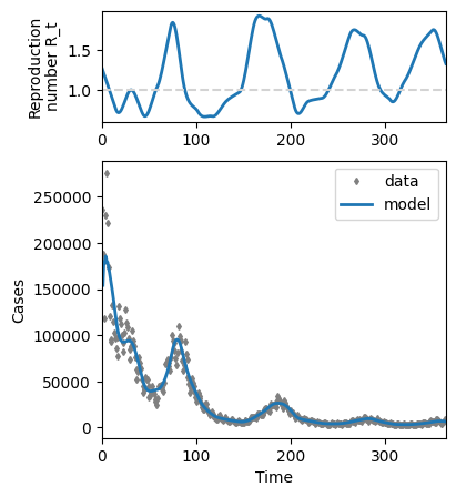
Let us check the results:
[7]:
f, axes = plt.subplots(2, 1, figsize=(4, 5), height_ratios=(1, 2.5))
plt.sca(axes[0])
plt.plot(
    t_out[:],
    simulation(res.params)["beta_t_interpolated"] * duration_infectious,
    color="tab:blue",
    label="model",
    lw=2,
)
plt.ylabel("Reproduction\nnumber R_t")
plt.xlim(t_out[0], t_out[-1])
plt.axhline([1], color="lightgray", ls="--")
plt.sca(axes[1])
plt.plot(t_out, data, color="gray", ls="", marker="d", ms=3, label="data")
plt.plot(
    t_out[1:],
    -np.diff(simulation(res.params)["S"]),
    color="tab:blue",
    label="model",
    lw=2,
)
plt.xlabel("Time")
plt.ylabel("Cases")
plt.legend()
plt.xlim(t_out[0], t_out[-1]);

Fitting using Adam#
For high-dimensional optimization systems that are significantly underdetermined it might be advantageous to use a gradient descent algorithm instead of L-BFGS. This is not the case for this system, but we show it here as an example using optax:
[8]:
start_learning_rate = 5e-2
schedule = optax.exponential_decay(
    init_value=start_learning_rate,
    transition_steps=1000,
    decay_rate=1 / 2,
    transition_begin=50,
    staircase=False,
    end_value=None,
)
optimizer = optax.adam(learning_rate=schedule)
# Initialize parameters of the model + optimizer.
opt_state = optimizer.init(init_params)
losses = []
params_adam = init_params
for i in (pbar := tqdm(range(2000))):
    func_val, grads = value_and_grad_loss(params_adam)
    if i % 10 == 0:
        pbar.set_description(f"Loss {func_val:.5f}")
    losses.append(func_val)
    updates, opt_state = optimizer.update(grads, opt_state)
    params_adam = optax.apply_updates(params_adam, updates)

f = plt.figure(figsize=(3, 2))
plt.plot(losses)
plt.ylim(1e3, 1e4)
plt.xlabel("iteration")
plt.ylabel("loss");
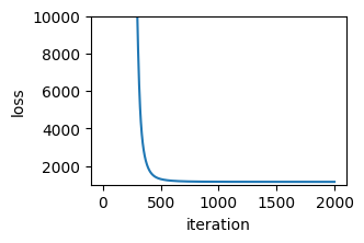
We obtain similar results:
[9]:
f, axes = plt.subplots(2, 1, figsize=(4, 5), height_ratios=(1, 2.5))
plt.sca(axes[0])
plt.plot(
    t_out[:],
    simulation(params_adam)["beta_t_interpolated"] * duration_infectious,
    color="tab:blue",
    label="model",
    lw=2,
)
plt.ylabel("Reproduction\nnumber R_t")
plt.xlim(t_out[0], t_out[-1])
plt.axhline([1], color="lightgray", ls="--")

plt.sca(axes[1])
plt.plot(t_out, data, color="gray", ls="", marker="d", ms=3, label="data")
plt.plot(
    t_out[1:],
    -np.diff(simulation(params_adam)["S"]),
    color="tab:blue",
    label="model",
    lw=2,
)
plt.xlabel("Time")
plt.ylabel("Cases")
plt.legend()
plt.xlim(t_out[0], t_out[-1]);
Bayesian analysis#
With fitting procedure one doesn’t obtain good error estimates of the fitted parameters. As such, a Bayesian model helps to estimate the credible interval of the parameters of interest. Let us make such a model for our system of equations.
The central part is the modelling of the infection rate beta_t. In a bayesian spirit, we assume that differences between subsequent knots of the spline interpolation follow an hierarchical model: We assume that the deviation of the size of changes in infectiousness is similar across the changes. The equations for the beta_t are therefore:
where \(\beta_k\) defines the k-th spline of the cubic interpolation. Let us define the model:
[10]:
# reduce the length of the simulation for runtime reasons
t_out_bayes = np.arange(100)
data_bayes = data[t_out_bayes]
t_solve_ODE_bayes = np.linspace(t_out_bayes[0], t_out_bayes[-1], len(t_out_bayes) // 2)
t_beta_bayes = np.linspace(t_out_bayes[0], t_out_bayes[-1], len(t_out_bayes) // 14)

# We therefore need a new ODEIntegrator object
integrator_object_bayes = icomo.ODEIntegrator(
    ts_out=t_out_bayes,
    ts_solver=t_solve_ODE_bayes,
    ts_arg=t_beta_bayes,
)

with pm.Model(coords={"time": t_out_bayes, "t_beta": t_beta_bayes}) as model:
    # We also allow the other rates of the compartments to vary
    duration_latent_var = pm.LogNormal(
        "duration_latent", mu=np.log(duration_latent), sigma=0.1
    )
    duration_infectious_var = pm.LogNormal(
        "duration_infectious", mu=np.log(duration_infectious), sigma=0.3
    )

    # Construct beta_t
    R0 = pm.LogNormal("R0", np.log(1), 1)
    beta_0_var = 1 * R0 / duration_infectious_var
    beta_t_var = beta_0_var * pt.exp(
        pt.cumsum(icomo.hierarchical_priors("beta_t_log_diff", dims=("t_beta",)))
    )

    # Set the other parameters and initial conditions
    const_args_var = {
        "N": N_England,
        "rate_latent": 1 / duration_latent_var,
        "rate_infectious": 1 / duration_infectious_var,
    }
    infections_0_var = pm.LogNormal(
        "infections_0", mu=np.log(data_bayes[0] * duration_infectious), sigma=2
    )

    y0_var = {
        "Es": [infections_0_var / 6 for _ in range(3)],
        "I": infections_0_var / 2,
        "R": 0,
    }
    y0_var["S"] = N_England - jax.tree_util.tree_reduce(lambda x, y: x + y, y0_var)

    # Define our integrator, notice that we use get_op instead of get_func. get_op
    # returns a pytensor operation that we can use in a pymc object.
    SEIR_integrator_op = integrator_object_bayes.get_op(
        Erlang_SEIR,
    )

    # And solve the ODE for our starting conditions and parameters
    output = SEIR_integrator_op(
        y0=y0_var, arg_t=beta_t_var, constant_args=const_args_var
    )
    pm.Deterministic("I", output["I"])
    new_cases = -pt.diff(output["S"])
    pm.Deterministic("new_cases", new_cases)

    # And define our likelihood
    sigma_error = pm.HalfCauchy("sigma_error", beta=1)
    pm.StudentT(
        "cases_observed",
        nu=4,
        mu=new_cases,
        sigma=sigma_error * pt.sqrt(new_cases + 1),
        observed=data_bayes[1:],
    )

    # Like before,w we also want to save the interpolated beta_t
    beta_t_interp = icomo.interpolate_pytensor(t_beta_bayes, t_out_bayes, beta_t_var)
    pm.Deterministic("beta_t_interp", beta_t_interp)
And then sample from it. We use the numpyro sampler, as it uses JAX which is more efficient as our differencial equation solver is written using jax. The normal pymc sampler also works. It would convert all the model in C, except our ODE solver, which would still run using JAX.
[11]:
trace = pm.sample(
    model=model,
    tune=300,
    draws=200,
    cores=4,
    nuts_sampler="numpyro",
    target_accept=0.9,
)
warnings = pm.stats.convergence.run_convergence_checks(
    trace,
    model=model,
)
pm.stats.convergence.log_warnings(warnings)
print(f"Maximal R-hat value: {max(az.rhat(trace).max().values()):.3f}")
Only 200 samples in chain.
Compiling...
Compilation time = 0:00:11.354689
Sampling...
Sampling time = 0:03:41.001574
Transforming variables...
Transformation time = 0:00:08.065634
The rhat statistic is larger than 1.01 for some parameters. This indicates problems during sampling. See https://arxiv.org/abs/1903.08008 for details
The effective sample size per chain is smaller than 100 for some parameters.  A higher number is needed for reliable rhat and ess computation. See https://arxiv.org/abs/1903.08008 for details
Maximal R-hat value: 1.040
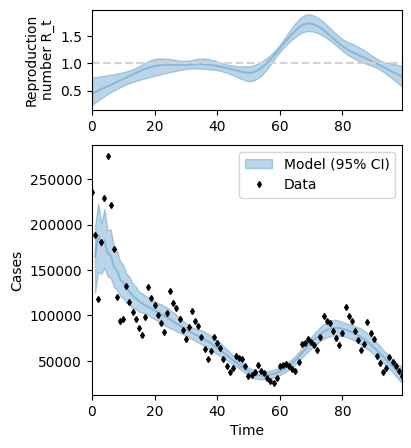
Notice how much longer the sampling takes compared to the simple fitting of the dynamics. It is also recommended to let it run for longer, to make sure the estimated posterior distribution converged. Let us plot the inferred parameters:
[12]:
f, axes = plt.subplots(2, 1, figsize=(4, 5), height_ratios=(1, 2.5))
plt.sca(axes[0])
beta_t_post = (
    trace.posterior["beta_t_interp"].to_numpy().reshape((-1, len(t_out_bayes)))
)
R_t_post = (
    beta_t_post * trace.posterior["duration_infectious"].to_numpy().flatten()[:, None]
)
plt.plot(t_out_bayes, np.median(R_t_post, axis=0), color="tab:blue", alpha=0.3)
plt.fill_between(
    t_out_bayes,
    *np.percentile(R_t_post, q=(2.5, 97.5), axis=0),
    color="tab:blue",
    alpha=0.3,
)
plt.ylabel("Reproduction\nnumber R_t")
plt.xlim(t_out_bayes[0], t_out_bayes[-1])
plt.axhline([1], color="lightgray", ls="--")

plt.sca(axes[1])
new_cases_post = (
    trace.posterior["new_cases"].to_numpy().reshape((-1, len(t_out_bayes) - 1))
)
plt.plot(
    t_out_bayes[1:], np.median(new_cases_post, axis=0), color="tab:blue", alpha=0.3
)
plt.fill_between(
    t_out_bayes[1:],
    *np.percentile(new_cases_post, q=(2.5, 97.5), axis=0),
    color="tab:blue",
    alpha=0.3,
    label="Model (95% CI)",
)
plt.plot(t_out_bayes, data_bayes, marker="d", color="black", ls="", ms=3, label="Data")
plt.ylabel("Cases")
plt.xlabel("Time")
plt.xlim(t_out_bayes[0], t_out_bayes[-1])
plt.legend();
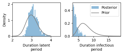
[13]:
f, axes = plt.subplots(1, 2, figsize=(5, 2.2))
x = np.linspace(1, 4, 100)
plt.sca(axes[0])
plt.hist(
    trace.posterior["duration_latent"].data.flatten(),
    bins=30,
    density=True,
    label="Posterior",
    alpha=0.5,
)
plt.plot(
    x,
    np.exp(pm.logp(pm.LogNormal.dist(np.log(duration_latent), 0.1), x).eval()),
    color="gray",
    label="Prior",
)
plt.xlim(2, 4.5)
plt.xlabel("Duration latent\nperiod")
plt.ylabel("Density")
plt.sca(axes[1])
x = np.linspace(3, 19, 100)
plt.hist(
    trace.posterior["duration_infectious"].data.flatten(),
    bins=30,
    density=True,
    label="Posterior",
    alpha=0.5,
)
plt.plot(
    x,
    np.exp(pm.logp(pm.LogNormal.dist(np.log(duration_infectious), 0.3), x).eval()),
    color="gray",
    label="Prior",
)
plt.xlim(3, 19)
plt.xlabel("Duration infectious\nperiod")
plt.legend()
plt.tight_layout();